
Introduction
Graph Neural Networks (GNNs) have emerged as a critical tool for modeling complex relationships and interactions in data, particularly in fields such as social and physical sciences. In this blog, we delve into the applications of GNNs in materials science (MS), an interdisciplinary field that combines elements of physics, chemistry, and engineering to understand and manipulate materials at the atomic and molecular levels. By capturing both local and global dependencies in graph-structured data, GNNs offer significant potential for advancing the discovery and development of new materials with desirable properties, as well as improving existing materials for various applications ranging from construction and electronics to healthcare and aerospace.

Graph Neural Networks
Graph Neural Networks (GNNs) are a class of neural networks that operate on graph structures. They have gained popularity due to their ability to model complex relationships and interactions in data that can be naturally represented as graphs, such as social networks, molecular structures, and materials.
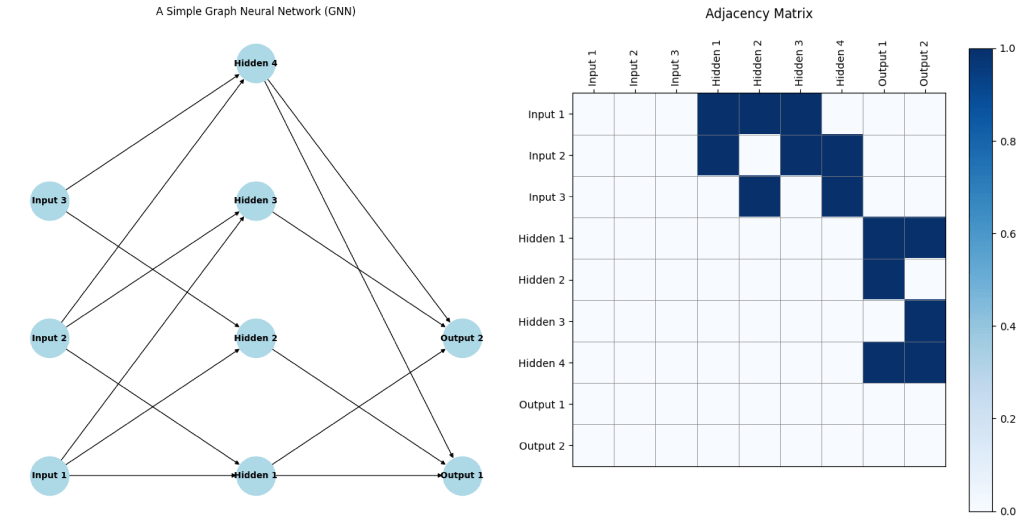
In a GNN, each node (or vertex) represents an entity, and each edge represents a relationship between entities. The GNN learns to propagate information through the graph, allowing it to capture both local and global dependencies. A critical component of GNNs is the adjacency matrix, which represents the connections between nodes in the graph. The adjacency matrix is a square matrix where each element indicates whether a pair of nodes is connected by an edge. This matrix is essential for defining the structure of the graph and for the operations that propagate information between nodes during the learning process.
GNN + MS
GNNs have emerged as one of the most powerful tools in MS due to their ability to naturally model the intricate relationships and interactions between atoms in a given material. Traditional machine learning approaches often struggle to capture the complexity of atomic interactions because they mainly rely on fixed grid-like structures, which are not well-suited for representing the irregular, non-Euclidean nature of molecular and crystal structures. GNNs, however, thrive in this domain as they operate directly on graph representations, where atoms are nodes and bonds are edges. This representation allows GNNs to efficiently capture both local interactions, such as covalent bonds, and global properties, like electronic band structures. By leveraging the inherent graph structure of materials, GNNs can predict and classify a wide range of properties, from mechanical strength to electronic behavior, enabling the discovery of new materials with tailored properties and accelerating the materials design process.
Implementation of GNNs for MS
Let’s dive into how we can use GNNs to model different materials. We’ll use Python and popular libraries such as PyTorch Geometric for our implementation.
Step 1: Setting Up the Environment
First, ensure you have the necessary libraries installed. You can install PyTorch and PyTorch Geometric using the following commands for Google Colab:
!pip install torch
!pip install torch-geometric
Step 2: Data Preparation
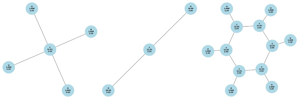
We’ll start by preparing our material data for methane (CH4), carbon dioxide (CO2), and benzene (C6H6).
Methane (CH4)
import torch
from torch_geometric.data import Data

# Methane (CH4) molecule
nodes_ch4 = torch.tensor([[6.0], [1.0], [1.0], [1.0], [1.0]], dtype=torch.float)  # Carbon and Hydrogen atoms
edges_ch4 = torch.tensor([[0, 0, 0, 0], [1, 2, 3, 4]], dtype=torch.long)  # Bonds between C and H
edge_attr_ch4 = torch.tensor([[1], [1], [1], [1]], dtype=torch.float)  # Single bonds
data_ch4 = Data(x=nodes_ch4, edge_index=edges_ch4, edge_attr=edge_attr_ch4, y=torch.tensor([16.0]))  # Example property
Carbon Dioxide (CO2)
# Carbon Dioxide (CO2) molecule
nodes_co2 = torch.tensor([[6.0], [8.0], [8.0]], dtype=torch.float)  # Carbon and Oxygen atoms
edges_co2 = torch.tensor([[0, 0], [1, 2]], dtype=torch.long)  # Bonds between C and O
edge_attr_co2 = torch.tensor([[2], [2]], dtype=torch.float)  # Double bonds
data_co2 = Data(x=nodes_co2, edge_index=edges_co2, edge_attr=edge_attr_co2, y=torch.tensor([44.0]))  # Example property
Benzene (C6H6)
# Benzene (C6H6) molecule
nodes_benzene = torch.tensor([[6.0], [6.0], [6.0], [6.0], [6.0], [6.0], [1.0], [1.0], [1.0], [1.0], [1.0], [1.0]], dtype=torch.float)  # Carbon and Hydrogen atoms
edges_benzene = torch.tensor([
    [0, 0, 1, 1, 2, 2, 3, 3, 4, 4, 5, 5, 0, 1, 2, 3, 4, 5],  # Bonds between C and H, and C-C
    [1, 6, 2, 7, 3, 8, 4, 9, 5, 10, 0, 11, 1, 2, 3, 4, 5, 0]
], dtype=torch.long)  # Bond indices
edge_attr_benzene = torch.tensor([[1], [1], [2], [1], [1], [2], [1], [2], [1], [2], [1], [1], [2], [1], [2], [1], [2], [1]], dtype=torch.float)  # Bond types
data_benzene = Data(x=nodes_benzene, edge_index=edges_benzene, edge_attr=edge_attr_benzene, y=torch.tensor([78.0]))  # Example property
Step 3: Defining the GNN Model
Next, we’ll define our GNN model. For simplicity, we’ll use a basic Graph Convolutional Network (GCN).
import torch.nn.functional as F
from torch_geometric.nn import GCNConv

class GCN(torch.nn.Module):
    def __init__(self, input_dim, hidden_dim, output_dim):
        super(GCN, self).__init__()
        self.conv1 = GCNConv(input_dim, hidden_dim)
        self.conv2 = GCNConv(hidden_dim, hidden_dim)
        self.fc = torch.nn.Linear(hidden_dim, output_dim)

    def forward(self, data):
        x, edge_index = data.x, data.edge_index
        x = self.conv1(x, edge_index)
        x = F.relu(x)
        x = self.conv2(x, edge_index)
        x = torch.mean(x, dim=0)  # Global mean pooling
        x = self.fc(x)
        return x

# Model instantiation
model = GCN(input_dim=1, hidden_dim=16, output_dim=1)
Step 4: Training the Model
We’ll now train the model on our material data. For simplicity, we’ll use the methane (CH4) data as an example.
import torch.optim as optim

# Training settings
learning_rate = 0.01
epochs = 100

# Optimizer
optimizer = optim.Adam(model.parameters(), lr=learning_rate)

# Training loop
model.train()
for epoch in range(epochs):
    optimizer.zero_grad()
    out = model(data_ch4)  # Change to data_co2 or data_benzene for other molecules
    target = data_ch4.y
    loss = F.mse_loss(out, target)
    loss.backward()
    optimizer.step()
    if epoch % 10 == 0:
        print(f'Epoch {epoch}, Loss: {loss.item()}')
Step 5: Evaluating the Model
Finally, we’ll evaluate the model’s performance.
# Evaluation
model.eval()
with torch.no_grad():
    prediction = model(data_ch4)  # Change to data_co2 or data_benzene for other molecules
    print(f'Prediction: {prediction.item()}, Target: {data_ch4.y.item()}')
Adding New Properties to the GNN
In our initial example, we only provided the atom numbers to the GNN as node features. However, it is possible to enhance the model by incorporating additional physical properties such as atomic mass and electronegativity. By doing so, we can provide the GNN with more detailed information about each atom, potentially improving the model’s performance. We can modify the code as follows:
Methane (CH4)
# Methane (CH4) molecule with atomic mass and electronegativity
# Node features: [atom_type, atomic_mass, electronegativity]
nodes_ch4 = torch.tensor([
    [6.0, 12.01, 2.55],  # Carbon atom: C
    [1.0, 1.008, 2.20],  # Hydrogen atoms: H
    [1.0, 1.008, 2.20],
    [1.0, 1.008, 2.20],
    [1.0, 1.008, 2.20]
], dtype=torch.float)
edges_ch4 = torch.tensor([[0, 0, 0, 0], [1, 2, 3, 4]], dtype=torch.long)  # Bonds between C and H
edge_attr_ch4 = torch.tensor([[1], [1], [1], [1]], dtype=torch.float)  # Single bonds
data_ch4 = Data(x=nodes_ch4, edge_index=edges_ch4, edge_attr=edge_attr_ch4, y=torch.tensor([16.0]))  # Example property
Carbon Dioxide (CO2)
# Carbon Dioxide (CO2) molecule with atomic mass and electronegativity
# Node features: [atom_type, atomic_mass, electronegativity]
nodes_co2 = torch.tensor([
    [6.0, 12.01, 2.55],  # Carbon atom: C
    [8.0, 16.00, 3.44],  # Oxygen atoms: O
    [8.0, 16.00, 3.44]
], dtype=torch.float)
edges_co2 = torch.tensor([[0, 0], [1, 2]], dtype=torch.long)  # Bonds between C and O
edge_attr_co2 = torch.tensor([[2], [2]], dtype=torch.float)  # Double bonds

data_co2 = Data(x=nodes_co2, edge_index=edges_co2, edge_attr=edge_attr_co2, y=torch.tensor([44.0]))  # Example property
Benzene (C6H6)
# Benzene (C6H6) molecule with atomic mass and electronegativity
# Node features: [atom_type, atomic_mass, electronegativity]
nodes_benzene = torch.tensor([
    [6.0, 12.01, 2.55],  # Carbon atoms: C
    [6.0, 12.01, 2.55],
    [6.0, 12.01, 2.55],
    [6.0, 12.01, 2.55],
    [6.0, 12.01, 2.55],
    [6.0, 12.01, 2.55],
    [1.0, 1.008, 2.20],  # Hydrogen atoms: H
    [1.0, 1.008, 2.20],
    [1.0, 1.008, 2.20],
    [1.0, 1.008, 2.20],
    [1.0, 1.008, 2.20],
    [1.0, 1.008, 2.20]
], dtype=torch.float)
edges_benzene = torch.tensor([
    [0, 0, 1, 1, 2, 2, 3, 3, 4, 4, 5, 5, 0, 1, 2, 3, 4, 5],  # Bonds between C and H, and C-C
    [1, 6, 2, 7, 3, 8, 4, 9, 5, 10, 0, 11, 1, 2, 3, 4, 5, 0]
], dtype=torch.long)  # Bond indices
edge_attr_benzene = torch.tensor([[1], [1], [2], [1], [1], [2], [1], [2], [1], [2], [1], [1], [2], [1], [2], [1], [2], [1]], dtype=torch.float)  # Bond types

data_benzene = Data(x=nodes_benzene, edge_index=edges_benzene, edge_attr=edge_attr_benzene, y=torch.tensor([78.0]))  # Example property
These modifications add the atomic mass and electronegativity as new physical properties to each atom node in the graph. This enhancement allows the GNN to leverage additional information, potentially leading to better performance in modeling and predicting material properties.
Conclusion
In this tutorial above, we’ve introduced materials science and graph neural networks, and demonstrated how to model different molecules using GNNs to make property prediction. This example provides a starting point for more complex and realistic applications, where you can experiment with different types of materials and GNN architectures for different type of tasks including classification and regression.
Stay tuned for more tutorials on advanced topics in materials science and machine learning!